OCR
Under the Hood: Visualizing a Convolutional Neural Network


Artificial Neural Networks (ANNs) are like black boxes. At Hypatos, we use them to extract machine readable information from documents to make back-office tasks more efficient...
Once the document is fed into the network, the black box spits out the information for us. The question that we try and address in this blog post is: How can we see inside this black box? Can we get any insights into the model by visualizing it?
ANNs should be thought of as graphs (not in the x-y axis interpretation that we have from school). We have nodes, where the data is stored, and edges, which represent a mathematical operation on the left-hand node to produce the value in the right-hand node along an edge. In this way, the data flows from left-hand side of the network to the right-hand side.
For example, if we input a line of a document, which is 16 words long (a bit small, but for the sake of simplicity) to detect whether the line is an address or not, the network may look something like this:

This architecture above is called a fully connected network – every node is connected to every node in the subsequent layer. Hypatos uses a more complicated network, especially convolutional layers. They are extremely useful for machine vision tasks (as discussed here) and allow the network to learn the 2D structure of the documents.
The mathematical operations that take place between the layers of the neural network have many unknown parameters. These are precisely the parameters that are fine-tuned by the network during the model’s training phase by passing labelled documents through it.
Once training is over, these parameters are fixed and new documents are passed through the network. The network will now automatically be able to extract the data that we are looking for.
This is great! However, we have no idea what all these nodes and edges of the network mean. For example, is one node looking for the word “Str.”? Is there another looking for a postcode? To do this, we have to understand the parameters that were fine-tuned. Convolutional layers are even harder, since they have kernels as parameters.
Visualization is difficult because the parameters are just numbers and have little meaning to the average human. To visualize this, we use the techniques of backpropagation¹ and guided backpropagation², which where first introduced to understand Convolutional Neural Networks (CNNs).
Backpropagation is a familiar term to those who have themselves trained a neural network. Assume we have a document that we have passed through the network during the training phase. The document is labelled so we can compare the output from the model with the actual labels that it should have outputted (the ground truth).
The model is given a way to measure the error between its output and the ground truth, usually called the loss. It is a number and the higher it is, the more erroneous the model is. Therefore, in order to make the model better, we “backpropagate” this loss through the fully connected and convolutional layers to the input layer calculating how sensitive the loss is to changes in parameters we want to fine tune.
Once this is done, the model changes the parameters (weights for fully connected layers and kernels for convolutional layers) so that the loss will now decrease. This process is repeated for the rest of the labelled documents until training is complete.
In order to create a visualization, instead of backpropagating through the network using a loss function we backpropagate the ground truth through the network. We end up with something with the same shape as the input, where each pixel is given a value that represents a word. This value measures the sensitivity of the ground truth with respect to the changes in the word in the pixel in question.

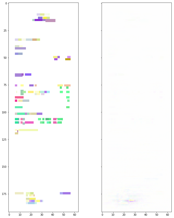
On the left we see a visualization of an invoice as the model sees it. On the right, we see the visualization after the backpropagation of the ground truth. We can immediately see from the dark region just above the first line on the right-hand image is important to the model. And this is not the only white space that the model deems to be important. The problem with this technique is that it is very noisy.
Guided backpropagation helps with this. It is similar to the vanilla backpropagation described above. However, in order to decrease the noise, we edit the way the network backpropagates through a specific layer type (the ReLU layers).

So far, the visualizations are in greyscale. There is a barrier to visualizing our model. Usually this technique is used on images, where the input has three color channels for each pixel. In our model, we have a word embedding that has 100 “color channels” for each pixel, which we cannot easily visualize. The technique used so far is to calculate the “length” of the word in each pixel, giving one number that we can give a greyscale value. We can use a dimension reduction technique called Principal Component Analysis (PCA) to help us.
PCA is a way of picking “the most important directions” in a space with a high dimension. In this case we pick the three most important directions out of the 100 possible given to us by the word embedding. Here are the color versions of the pictures above.

Too noisy!

That’s better.
The pictures above show the sensitivity of the whole ground truth to changes to the words in each pixels. We can also backpropagate specific items that we are interested in to see what pixels are important to the model for that particular item.
Here, we have a visualization of guided backpropagation of the IBAN item on this invoice. Can you guess where it is located on the raw invoice on the left hand side? It’s not so easy: it could be any of the lines at the bottom of the invoice on the left. Most likely the second to last line (which it is).

This is a visualization of guided backpropagation of the VAT identification number. Here, it’s much easier to identify the VAT identification number on the left-hand image.
From this one example, we can already see that the model is a lot more confident about the location of the VAT identification number in comparison to IBAN.
Hypatos is working hard to improve our model and this technique is an exciting avenue that we will continue to explore.
[²] Striving for Simplicity: The All Convolutional Net – Jost Tobias Springenberg, Alexey Dosovitskiy, Thomas Brox, Martin Riedmiller
Further stories from our blog
.jpg)


